Chapter 1 Introduction: Getting Familiar with R and RStudio
1.1 What is R and RStudio?
R is a language and environment for statistical computing, based on the S language developed at Bell Labs. It supports both classical and modern statistical analysis and is free to use. A core team and contributors maintain R across major operating systems. Visit http://www.r-project.org for more information.
We won’t use R directly. Instead, we’ll use RStudio, a free integrated development environment (IDE) that makes interacting with R easier. Think of R as the engine and RStudio as the dashboard—it helps control and extend R’s capabilities, like creating documents, apps, and more.
1.2 Downloading and Installing R
You can use R and RStudio via the CSUB virtual lab. To install them on your own computer:
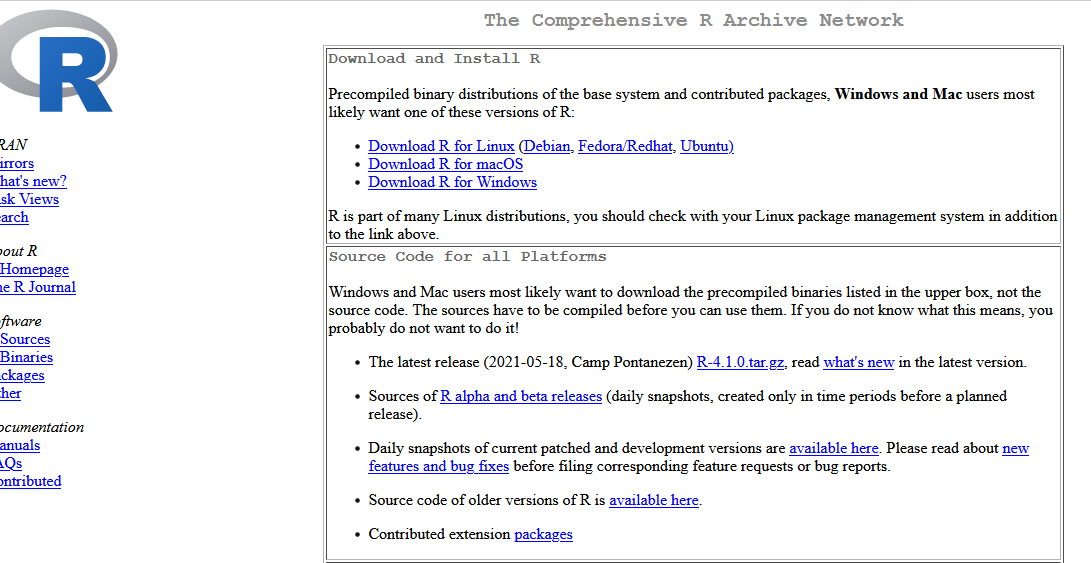
- Go to https://cran.r-project.org/.
- Select your operating system (see Figure 1.1).
- Click base, then download the latest version.
- Run the installer using default settings.
- Done!
1.3 Downloading and Installing RStudio
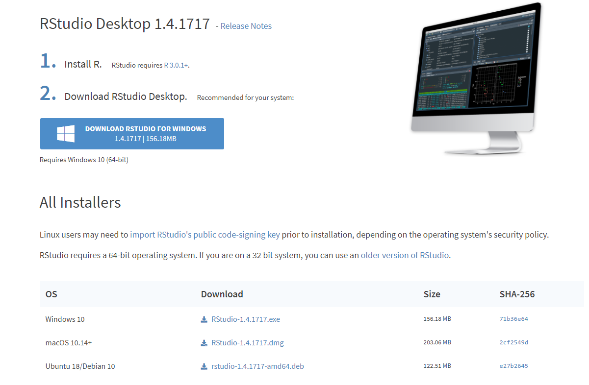
- Visit http://www.rstudio.com/products/rstudio/download/ and scroll to “RStudio Desktop” (Figure 1.2).
- Click “DOWNLOAD” and select your OS version (Figure 1.3).
- Run the installer using default settings.
- Done! Launch RStudio from your computer.

1.4 Layout of RStudio
Open RStudio. You’ll see three panes by default (Figure 1.4). A fourth opens when you go to File > New File > R Script.
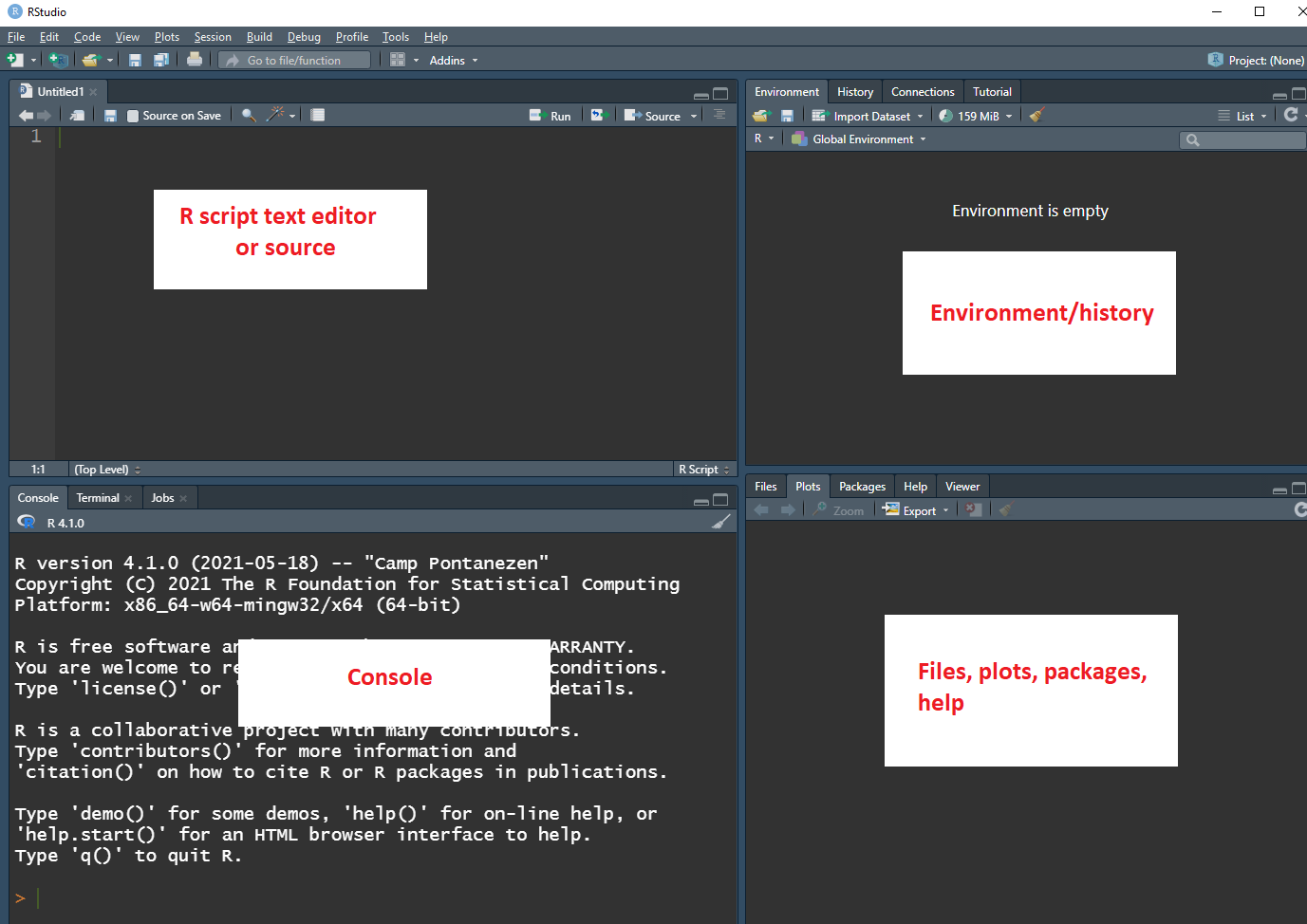
Panes overview:
- Top-left: Script editor (source) for writing reusable R code.
- Bottom-left: Console where commands run and output appears.
- Top-right: Environment (data in memory) and History (past commands).
- Bottom-right: Tabs for Files, Plots, Packages, and Help.
1.5 Expressions and Assignments
Try the following in the console:
25 - 5(expression)h = 25 - 5(assignment)hH <- 20; thenH
Key points:
- R is case sensitive:
h\(\neq\)H. - Created objects appear in the Environment tab.
- Objects persist only during a session unless saved.
- Use
=or<-for assignment. People tend to prefer<-. - Object names must start with a letter and can include letters, numbers, or periods (no spaces).
#marks a comment (ignored by R).
To quit, use File > Quit Session or type q().
1.6 Running R Code in RStudio
To enter code efficiently:
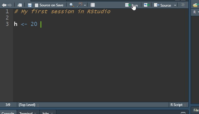
- Open a new script (File > New File > R Script).
- Type code (e.g.,
h <- 20). - Save it as an
.Rfile (e.g., FirstRsession.R). - Highlight a line and click “Run” to execute it.
Tip: Save your script regularly.
1.7 A Fancy Calculator
R handles basic math:
Output:
[1] 4.4601227
Other examples:
Notes:
>means R is ready.- Spacing doesn’t matter (
5/2\(=\)5 / 2), but improves readability.
## Working with Vectors

Combine values into a vector using `c()`:


``` r
x <- c(1, 0, 2, 0, 3)
x
## [1] 1 0 2 0 3Calculate mean:
## [1] 1.2Or use built-in functions:
## [1] 6## [1] 1.2To compute sum of squares:
## [1] 1 0 4 0 9## [1] 14To compute variance-like quantity:
## [1] -0.2 -1.2 0.8 -1.2 1.8## [1] 1.71.8 Data Types in R
Key types:
- Numeric
- Character (strings)
- Logical (TRUE/FALSE)
- Factor
Examples:
## [1] 10.355## [1] "hi" "hello"## [1] "3.4403"## [1] TRUE TRUE FALSEMaritalStatus <- c("married", "married", "divorced", "single", "single", "widowed", "married")
MaritalStatus## [1] "married" "married" "divorced" "single"
## [5] "single" "widowed" "married"## [1] married married divorced single single
## [6] widowed married
## Levels: divorced married single widowedVectors can only contain one type. Recognizing data types is more important than creating them.
1.10 Using R Functions
Use c() to create a vector:
Use arrow keys to recall past commands. Built-in functions like sum() are common:
1.11 Loading and Installing Packages
R comes with base packages. Some, like mean(), are loaded by default. Others, like boxcox() from MASS, must be loaded manually:
Install additional packages once using:
Follow prompts (choose USA mirror, allow personal library, update if asked). After installation, load packages in each session using library(openintro) or require(openintro).
1.9 Comments in R
Use
#for comments:Use comments to clarify code.